Why using R-squared is a bad idea

21 Nov 2015

The coefficient of determination is otherwise known as \(R^2\) and is often used to determine whether a model is good. The Wikipedia article says that \(R^2\) “[…] is a number that indicates how well data fit a statistical model – sometimes simply a line or a curve. An \(R^2\) of 1 indicates that the regression line perfectly fits the data, while an \(R^2\) of 0 indicates that the line does not fit the data at all”. From this we could conclude that we can use this measure to indicate how good our model is. There are, however, 2 major problems with that conclusion:

Sometimes just having a model that is a little better than random guessing is already great.
Adding useless covariates to the model improves \(R^2\).

The first argument is supported best by the example stock market. If I have a model that is just a little bit better than random guessing, I will be rich. The second argument I want to show on an example.

set.seed(17)

n <- 200

x <- rnorm(n = n, mean = 1, sd = 1)
y <- 2 + 5 * x + rnorm(n = n, mean = 0, sd = 20)
df <- data.frame(y = y, x = x)

lmod <- lm(y ~ x, data = df)
summary(lmod)

## 
## Call:
## lm(formula = y ~ x, data = df)
## 
## Residuals:
##     Min      1Q  Median      3Q     Max 
## -63.303 -12.432  -0.923  12.558  58.839 
## 
## Coefficients:
##             Estimate Std. Error t value Pr(>|t|)    
## (Intercept)    1.336      1.838   0.727    0.468    
## x              6.749      1.271   5.310 2.94e-07 ***
## ---
## Signif. codes:  0 '***' 0.001 '**' 0.01 '*' 0.05 '.' 0.1 ' ' 1
## 
## Residual standard error: 19.63 on 198 degrees of freedom
## Multiple R-squared:  0.1246,	Adjusted R-squared:  0.1202 
## F-statistic: 28.19 on 1 and 198 DF,  p-value: 2.935e-07

summary(lmod)$r.squared

## [1] 0.1246397

So we have an outcome \(y\) that depends on a covariate \(x\), but the noise is very high, so our \(R^2\) is pretty low. Let’s add further useless covarates to the model.

R2 <- data.frame(p_useless = NULL, R2 = NULL, adjusted = NULL)

for(i in 1:(n-1)) {
  j <- ncol(df)
  df[ , j+1] <- rnorm(n = n, mean = 0, sd = 1)
  tmp <- data.frame(p_useless = i,
                    R2 = c(summary(lm(y ~ ., data = df))$r.squared)
  )
  R2 <- rbind(R2, tmp)
}

library(ggplot2)
ggplot(data = R2, aes(x = p_useless, y = R2)) + 
  geom_point() + 
  ylab(expression(R^2)) + 
  xlab("number of useless covariates")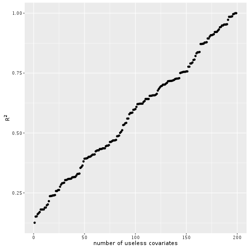

And voilà the more random covariates we add the better the model according to \(R^2\). Does not make sense right?

Heidi's stats blog

Why using R-squared is a bad idea